Virtual SIPs

The Generator Generator

by Sam L. Savage

GeneratorGenerator.png
 

Distribution Distribution

Decades ago, I discovered that few managers were benefiting from probabilistic analysis. Despite widely available simulation software such as @RISK and Crystal Ball, most people lacked the statistical training required to generate the appropriate distributions of inputs. 

“But wait a minute,” I thought to myself. “The general public still uses light bulbs even though they don’t know how to generate the appropriate electrical current.” After some research I discovered that there is a power distribution network that carries current from those who know how to generate it to those who just want to use it.

So why not create a Distribution Distribution network, to carry probability distributions from the people who know how to generate them (statisticians, econometricians, engineers, etc.) to anyone facing uncertainty?

Great idea, but it took me a while to figure out the best way to distribute distributions.  Eventually I arrived at the SIPs and SLURPs of probability management, which represent distributions as vectors of realizations and metadata which support addition, multiplication, and any other algebraic calculation, while capturing any possible statistical relationship between variables. This concept even works with the data set invented by Alberto Cairo, made up of SIPs I call Dino and saur [i].

A Scatter Plot of Alberto Cairo’s Dino and saur

A Scatter Plot of Alberto Cairo’s Dino and saur


Once Excel fixed the Data Table, it became possible to process SIPs in the native spreadsheet, which greatly accelerated adoption [ii]. SIPs and SLURPs have been a simple, robust solution, although they do require a good deal of storage.

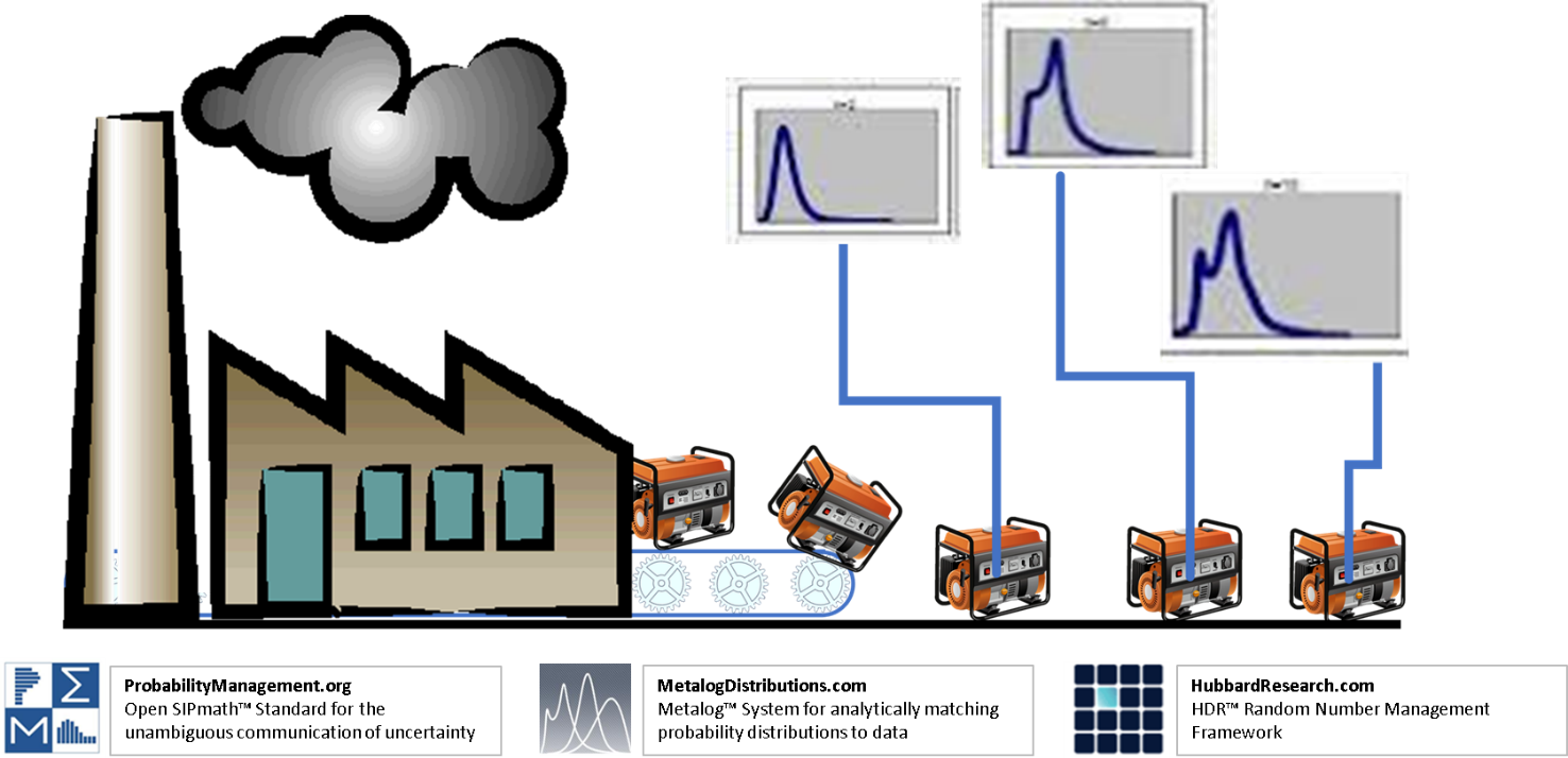
Before I thought of SIPs, I had thought of and abandoned an idea involving snippets of code which would generate a random number generator when they arrived on a client computer.  I called this approach the Generator Generator (well, that was for short—the full name was the Distribution Distribution Generator Generator). The advantage of such a system is that the storage requirements would be tiny compared to SIPs, and you could run as many trials as you liked. It might not be possible to capture the interrelationships of Dino and saur, but at least some forms of correlations could be preserved.

The SIPmath/Metalog/HDR Integration

Recent breakthroughs from two comrades-in-arms in the War on Averages have made the Generator Generator a reality and allowed it to be incorporated into the SIPMath Standard. One key ingredient is Tom Keelin’s amazingly general Metalog System for analytically modeling virtually any continuous probability distribution with one formula.

Another is Doug Hubbard’s latest Random Number Management Framework, which in effect can dole out independent uniform random numbers like IP addresses while maintaining the auditability required by probability management. This guarantees that when global variables such as GDP are simulated in different divisions of an organization, they will use same random number seed. On the other hand, when simulating local variables, such as the uncertain cost per foot of several different paving projects, different seeds will be guaranteed. This allows individual simulations to be later aggregated to roll up enterprise risk. Doug’s latest generator has been tested thoroughly using the rigorous dieharder tests [iii].

At ProbabilityManagement.org, we have wrapped these two advances into the Open SIPmath Standard for creating libraries of virtual SIPs, which will take up a tiny fraction of the storage of current SIP libraries. We hope to release the tools to create such libraries at our Annual Meeting in San Jose on March 26 and 27. Tom, Doug, and I will be presenting there, along with an all-star cast of other speakers. I hope we see you there.

© Copyright 2019, Sam L. Savage

All-Star Lineup for our 2019 Annual Conference

loring_ward_3.jpg

by Sam Savage

Applications of Probability Management
March 26 - 27, 2019
San Jose, CA

SIPmath is a broad-spectrum cure for the Flaw of Averages, which impacts all plans involving uncertainty. With this in mind, our 2019 Annual Conference casts a wide net over a variety of probability management applications. I urge you to look through the abstracts.

 We have many great speakers lined up, including:

  • Deborah Gordon – Director, City/County Association of Governments, San Mateo County

  • Max Henrion – CEO of Lumina Decision Systems and 2018 Ramsey Decision Analysis Medal Recipient

  • Doug Hubbard – author of How to Measure Anything and The Failure of Risk Management

  • Tom Keelin – Inventor of the Metalog Distribution & Chief Research Scientist at ProbabilityManagement.org

  • Michael Lepech – Associate Professor of Civil and Environmental Engineering, Stanford University

  • Harry Markowitz – Nobel Laureate in Economics (via live webcast)

  • Greg Parnell – Military Operations Researcher & Professor at the University of Arkansas

  • Stan Uryasev – Risk Management Expert & Professor at the University of Florida

Topics covered include:

  • Analytics Wiki Development

  • Applying in SIPmath in Human Relations

  • Military Readiness

  • Municipal Risk Management

  • Applied Economics

  • Probabilistic Energy Forecast

  • Bridge Safety

  • Water Management

Register by Friday, February 1 to take advantage of our early registration discount.

Video Excerpts: Probability Management at Stanford University

SCPD Logo.png
 

by Sam Savage

On September 17, I delivered a one-hour webinar previewing my Winter Quarter course in Project Risk Analysis in Stanford University’s Department of Civil and Environmental Engineering. This course will apply the discipline of probability management to such problems as risk return tradeoffs in R&D portfolios and rolling up operational risk across assets such as gas pipelines. Although the entire 57-minute webinar is available, I recommend the following excerpts.


The "Chance of Whatever" Button

Defense against “Give me a Number”

by Sam Savage

ChanceofWhateverArrow.png

A common fork in the road to hell is arrived at when, in the face of uncertainty, the boss demands: “Give me a number.” You may be tempted to respond with, “Would you settle for an average?” But even the correct average of the uncertain duration of a task, demand for a new product, or labor hour requirements for a job, leads to a host of systematic errors that guarantee that your plans will be wrong on average. I dubbed this problem “The Flaw of Averages” in an article in the San Jose Mercury News in 2000, and have been struggling to correct it ever since with growing success.

Technically you should say to the boss, “Here’s the probability distribution of the number you want.” But I don’t recommend that if you want to keep your job. Instead, the latest version of the SIPmath™ Modeler Tools, both the free version and guilt-free $500 Enterprise version, now include the new “Chance of Whatever” button.

Just put your cursor in the cell where you want the chance of whatever to appear, then specify the uncertain cell that needs to be greater or less than your boss’s specified goal. Then click OK. Now as you change your goal, the chance cell will immediately update. So, next time the boss demands a number, you can respond with, “What do you want it to be? I can tell you the chance of meeting your goal.”

Brian Putt, Chair of Energy Practice at ProbabilityManagement.org, has a new video on how to use this feature of our tools. Check it out.


© Copyright 2018 Sam Savage

Tom Keelin Named Chief Research Scientist

by Sam Savage

Tom Keelin

Tom Keelin

We are happy to announce that Tom Keelin, inventor of the Metalog system, will join ProbabilityManagement.org as Chief Research Scientist. Tom is Founder and Managing Partner at Keelin Reeds Partners, former Worldwide Managing Director of Strategic Decisions Group, and co-founder of Decision Education Foundation. He holds a PhD in Engineering-Economic Systems from Stanford University.

On their own, Metalogs represent an unprecedented, unified approach to creating analytical formulas to represent probability distributions derived from data. Coupled to the HDR Random Number Management Framework from Doug Hubbard, they are leading to a new generation of SIPmath in which SIP libraries, which currently may contain millions of data elements, will be reduced to a few lines of code. These in turn will create virtual SIPs on an as-needed basis, without losing the fundamental properties of additivity and auditability that are the hallmarks of the discipline of probability management.

Watch for an upcoming blog post on the combined use of the SIPmath, HDR, and Metalog standards.

Related Reading: Tom Keelin’s Metalog Distributions

© Copyright 2018 Sam Savage

None of My Successes Have Been Planned and None of My Plans Have Been Successful

Simulating Rags to Riches and Vice Versa

by Sam Savage

Blog_HeatMap.png
 

Planning vs. Scheming

Since much of my income is from consulting, I have devoted resources to reaching out to appropriate clients. I can’t count the number of engagements I’ve gotten this way because there aren’t any. All my engagements have dropped in from out of the blue.

“But how about your 2009 book?” you say. “That was marketing on a grand scale. Some would have even called it selling out. You must have had customers breaking down your door after that.”

Nope. There was a horrific worldwide recession and I lost my key clients instead of getting new ones.

“But things are going great now, right?” Absolutely, and I am deeply thankful. But this was due to dumb luck, such as the improved Data Table function in Microsoft Excel, which enabled SIPmath, and stumbling upon adult supervision in the nick of time.

None of my successes have been planned and none of my plans have been successful. So, I don’t plan (much to the consternation of my adult supervisors). Instead, I scheme, by putting options in place in case the appropriate planets align. However, Louis Pasteur said that “Chance favors the prepared mind,” and I do try to prepare my mind. I just don’t plan.

So, when I heard that three Italian physicists (Pluchino, Biondo, & Rapisarda) had written a paper called “Talent vs Luck: the role of randomness in success and failure,” I was all ears. Among other things, they address the question of why, if talent is distributed along a bell curve, that wealth is extremely skewed with the top few percent of the population owning the lion’s share. They created a simulation that shows how chance drives the disparity in the distributions of talent and wealth. Inspired by the physicists, Dave Empey [1] and I built our own SIPmath model in Excel (available on our Models page) to explore similar principles. Our model shows that chance plays a role, but that disparity in income can arise without it. NOTE that unlike the physicists’ model, ours is not calibrated to reality, and is merely designed to give directional results.  

The Model

Free models, like free advice, are worth what you pay for them. The admonition of George Box, that “all models are wrong, but some are useful,” applies in spades to economics, where Chaos Theory is always lurking a few decimal places away. I think the Italians would agree with me that such models do not provide “right answers” as much as “right questions.”


With the above caveats in mind, our model has the following elements.

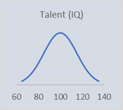
1. We start with 50 agents, whose talents are measured in IQ score, normally distributed with mean of 100 and standard deviation of 15. These are assigned at the beginning and do not change during the simulation.

Blog_Talent.png
Blog_Wealth.png
 

We also endow the agents with an initial wealth distribution, which may be uniform, or skewed either toward the high or low intelligence agents.

Blog_Additive.png

2. . We then simulate two forms of IQ-based income (wealth accumulation) over twenty years; either adding wealth proportional to IQ or multiplying wealth by a factor proportional to IQ. In either case the user may specify a degree of uncertainty from year to year.

3. We also allow for additional Chance Events that can impose independent positive or negative impacts for each agent.

Blog_HeatMap2.png

4. A heatmap displays the relative wealth by year each agent for a single trial. It is fun to crank up the uncertainty, press the <calculate> key, and watch the unsuspecting agents succeed or fail beyond their wildest simulated dreams.

5. Given the above calculations, we run 100 simulated trials of final wealth for each of the 50 agents, effectively generating a simulated population of 5,000 agents over which we calculate the final wealth distribution.

Results

A key result of Pluchino, Biondo, & Rapisarda is that the final wealth in their simulation (which was more complex than ours) was very skewed even though talent was normally distributed.  Our model indicates that you can’t sneeze without creating a skewed distribution of final wealth. For example, suppose there is no uncertainty, and all agents start with equal wealth, that increases each by a percentage proportional to their IQ. This is analogous to agents with investments that grow at different rates. Then you get the distribution of final wealth shown below.  

Blog_FinalWealth.png
Blog_PercentofWealth.png

Here we have the top 1% of the population holding 10% of the wealth. Adding additional uncertainties makes the skew worse, but talk is cheap, I suggest that you download the model here and play with it yourself.


[1] Director of Software Development at ProbabilityManagement.org and programmer of the SIPmath™ Modeler Tools.

© Copyright 2018 Sam Savage

Unambiguous Uncertainty

Cards.png

by Sam Savage

The other night I was reading Behave, Robert Sapolsky’s magnificent book on human behavior, when something grabbed my attention. On page 35, Sapolsky describes two psychological experiments. In the first experiment, the subject is presented with a deck of cards, is told that half are red and half are black, and asked how much they would wager that the top card is red. Because there is an even chance of the top card being red or black, the risk-neutral bet (that is, the maximum payment you would make for a wager that pays you $1 if you win) would be 50 cents.

In the second experiment, the subject is told that the deck consists of red and black cards, and has at least one red and at least one black card. When the subject is asked to consider the same wager as before, again the risk-neutral bid is 50 cents because neither red or black is more likely to appear than the other.

amygdala.png

So, what’s the difference between these two experiments? In the second one, the subject’s amygdala (the emotional center of the limbic system, which triggers the fight or flight response) lights up like a Christmas tree when viewed with functional MRI! The explanation for this strong reaction is that the ambiguity of the second deck induces anxiety[1]. The subject knows there is one red and one black card, but what are the rest of the cards? Experiments like these bring scientific rigor to the emerging field of Behavioral Economics.

The relevance to probability management is that in our discipline, uncertainty is communicated in SIPs (Stochastic Information Packets), which are randomly shuffled potential outcomes similar to the first deck of cards. With SIPs, the uncertainty is unambiguous. You can take your time and look at each number in advance, which is comforting, but you know only one will be selected when the uncertainty is resolved. This is unlike traditional simulation, which generates random experiments on the fly, thereby driving accountants bonkers. Instead, SIPs contain metadata, including provenance, so you know that they are not just something the cat dragged in. Then, when the accountants come knocking, you can say, “We are basing our decision on fifty million deterministic numbers. How about auditing these for us?” That’ll get them off your back for a few days.

This discussion also highlights the difference between the two famous feuding schools of probability, the frequentists and the Bayesians. The frequentists define the probability of an event as the proportion of times the event occurs in a large number of identical experiments. For example, if you actually wagered on Red over a thousand standard shuffled decks, you would win about 500 times, and the relative probability of red to black would be defined as 50%. A true frequentist might have trouble with deck two because they would not know how to define the repeatable experiment. The Bayesians, for whom my father was a major evangelist, think of probability as being subjective, and determined by the risk-neutral wager you would make on the outcome. Bayesians have no problem putting a relative probability of 50% on the outcomes of experiment two, which suggest that perhaps members of the two schools could be identified by what their amygdalae do in MRI machines.

Uncertainty Light

In his book The Black Swan, Nicholas Taleb coined the term Ludic Fallacy to warn against "the misuse of games to model real-life situations." His warning should be heeded. However, I define the Ludic Fallacy-Fallacy to be the belief that you can manage real-life uncertainties without first understanding the simple arithmetic of dice, cards, and spinners. One thousand auditable potential outcomes may not contain any black swans, but it is way better than the industry standard of using a single average number to represent an uncertain future.

And speaking of games, an associate’s son is a star Little League baseball player. During the regular season his team dominated the other local teams, composed of kids he had known and played against for years. They easily made it into the playoffs with teams from other cities. At that point, facing the ambiguity of the unknown opposing players, his mother told me that the poor kid’s amygdala went up in flames of pre-game anxiety. They made it all the way through the playoffs, finally losing in a tight game in the fourth and final round. I asked if his anxiety had persisted during the championship play, and was told that by the second game “he had learned to play with deck two.”

So, think of probability management as “Uncertainty Light,” designed to calm those with Post Traumatic Statistics Disorder during the regular season. But don’t be lulled into complacency. You’ll never make the playoffs if you can’t deal with the ambiguity of the second deck.  

To learn probability management applications, sign up for our Fort Worth workshop or an upcoming webinar. 


[1] Doug Hubbard, author of the popular How to Measure Anything series, uses a variant of the card experiment called the Urn of Mystery, which shows the importance of drawing even a single sample before you wager in case 2 above. You may download Doug’s Urn simulation here.

© Copyright 2018 Sam Savage


The Sum of the Sandbags Doesn’t Equal the Sandbag of the Sum

How Probability Management Helps Solve Age-Old Problems in Budgeting and Forecasting

by Sam Savage

Sandbags.png

Sandbagging is the practice of padding one’s budget to avoid running out of money in the face of an uncertain forecast. Suppose, for example, that ten managers each have independent uncertain annual expenditures that average $10M. Let’s assume they all cover their butts by forecasting the 90th percentile, which turns out to be $11M (the Sandbags). Now they each have only a 10% chance of blowing their budget.

Next, the CFO rolls these forecasts up to get $110M (the Sum of the Sandbags). And suppose the enterprise can also tolerate a 10% chance of exceeding the overall budget. The problem is that due to the diversification effect, there is only about one chance in 1,000 that the CFO will blow through all $110M. Why? Suppose one manager, Paul, ends up exceeding his budget at the end of the year, while another, Peter, has extra cash. Then the CFO can borrow from Peter to pay Paul, and all is well. So mathematically, given the options to balance across the portfolio at the end of the year, the 90th percentile at the line item level turns into something like the 99.99th percentile at the enterprise level.

To achieve the desired 90% confidence, the CFO might need only $105M, which we refer to as the Sandbag of the Sum. So, in this case, $5M is just lying around gathering dust instead of being available as investment capital. If you don’t think that’s a big deal, go out and try raising $5M sometime. And this problem only compounds as you roll up layers upon layers of fat through a multi-tiered organization. In the above, and most examples, the Sum of the Sandbags is greater than the Sandbag of the Sum (the number you should budget at the portfolio level given your organization’s risk tolerance). But the inequality can sometimes go the other way with asymmetric distributions, and you can’t do this stuff in your head.

When I wrote the first edition of The Flaw of Averages, there was no practical way to solve this problem on a universal scale. Today, however, thanks to the Open SIPmath™ Standard, anyone with a spreadsheet can easily perform the necessary calculations with uncertain budgets. What remains is the re-alignment of the numerous stakeholders involved. Impossible, you say? Someone who has done this the hard way without SIPmath is Matthew Raphaelson, who first introduced me to the Sandbag Problem years ago. Matthew is a former senior banking executive with 25 years of experience, which includes being CFO of a large business unit. He is also chair of Banking Applications at ProbabilityManagement.org.

He stresses that some managers may use probability as an excuse for lack of accountability. “At the end of the day,” says Matthew, “managers – not machines – need to own their forecasts and be accountable for their results.”  He warns that “a company that relies solely on centralized models will be met with smirks and shrugs when it attempts to distinguish between forecast errors and performance misses.”

Matthew, who has been on the front lines of numerous budget wars, describes five stages of managerial development for tackling the sandbag issue.

  1. Education
    Make managers aware of the problem, and how today there is a practical solution.

  2. Communication
    Understanding percentiles, and communicating uncertain estimates as auditable data.

  3. Models and Data
    Convert existing data infrastructures to handle SIP libraries instead of numbers. This is no big deal and can be done with current software.

  4. Incentives and Cultural Change
    The “nobody gets in trouble for beating a forecast” mentality is the root cause of the sandbagging problem. Gamification can both provide new incentives and train managers to become better forecasters in the face of uncertainty.

  5. Analysis and Action
    Once uncertainty becomes auditable, it may be systematically reduced in a continual improvement process.

Matthew and I have written on this subject for the Banking Administration Institute (BAI).

And there are two separate documented SIPmath models available below that perform thousands of simulation trials per keystroke to connect the seat of your intellect to the seat of your pants.

SandbagCalc Demonstrates basic sandbag math

SandbagCalc
Demonstrates basic sandbag math

Model from BAI article Banking example with revenues and expenses

Model from BAI article
Banking example with revenues and expenses

I will end with a war story from Matthew, which foretells the nature of the battle ahead.

“In the 1990s, I asked managers to give me a ‘50th percentile’ forecast to avoid the sandbag problem.  Apparently, this guidance wasn't as clear as it needed to be.  One manager's monthly expense results kept coming in lower than forecast, to the point where it was clear there had to be some bias.  I re-affirmed with the manager that he provided 50th percentile forecasts.  ‘Oh, absolutely,’ he said.  Probing a bit, I asked if this meant there was a 50% chance that actual expenses would come in lower than forecast each month. ‘Yes, that's what it means,’ he said.  And so, is there also a 50% chance that actual expenses would come in higher than forecast each month?  ‘Oh no, there is almost no chance of exceeding our forecast....’”

© Copyright 2018 Sam Savage

Tom Keelin's Metalog Distributions

Mathematical Elegance Coupled to Computational Efficiency

by Sam Savage

Metalog.jpg

After receiving his PhD in Decision Analysis from Stanford, Tom spent 40 years in analytical consulting, including an 18-year stint at the prestigious Strategic Decisions Group, where he was Worldwide Managing Director. Tom was struck by general management’s inability to compute uncertainties, and has developed a flexible family of continuous data-driven probability distributions based on pragmatic consulting experience. The Metalog distributions, as he calls them, combine mathematical elegance with computational efficiency [i], [ii], [iii].

To put Metalogs in perspective, I remind the reader that the theory of probability and statistics is powerful and elegant. But so is the steam locomotive, and they were developed around the same time. By the 1970’s, computational approaches to statistics such as bootstrapping arose. These were based on the brute force of computer simulation instead of 19th century calculus. Although Metalogs are also based on simple mathematical principles, they are intended to be fit to data sets, not adjusted by parameters such a mean and standard deviation.  And they output the ideal food for simulations:  inverse cumulative functions. These functions are the most common way to generate random variates in simulations. The Excel function NORMINV(rand(),Mean,Sigma), for example, will produce Normal random variables with the specified mean and standard deviation with every press of the Calculate Key.

The informative Metalog Distributions website contains extensive documentation and implementations in numerous environments, including Excel and R. We have already implemented some of the Metalogs in the SIPmath™ Modeler Tools as described below. You can also download any of the Excel templates from the Metalog website and use them with the tools. Just be sure to replace the “random” cells in the templates with either RAND() or HDR generators from the SIPmath tools.

It is still early innings for Metalogs. For example, last year Tom and I discovered how to generalize the concept to solve a vexing problem in simulation. Suppose you are modeling an uncertain number of risk events, such a transformer failure. Each failure will cause a fire with a skewed, lognormally, distributed adverse consequence. On a given simulation trial you may get 3, 5, 8 or some other number of failures, and need to add up 3, 5, 8 or some other number of lognormal distributions. But you don’t know in advance how many you will have so you don’t know how many you need to generate. Until our approach with the Generalized Metalog, there was apparently no closed form solution for expressing sums of lognormals. We (mostly Tom) wrote this up for publication, and with his help we built sums of lognormal and triangular distributions into the Enterprise SIPmath™ Modeler Tools. Tom is now Chair of Data-Driven Distributions at  ProbabilityManagement.org, and we will keep you apprised of future Metalog developments, several of which are in progress.

Using Metalogs in the SIPmath Tools

All the latest versions of the tools support the SPT (symmetric percentile triplet) Metalog, which can produce a wide range of distribution shapes as shown below [iv].

Metalog1.png


Furthermore, Tom has written a nice tutorial on their use in the SIPmath Tools.

The sums of identical triangular and lognormals are implemented in the Enterprise version of the tools, as described below.

Sum of Lognormal Risk Consequences in the SIPmath Tools

Suppose your organization is subject to a risk characterized by an average of 5 adverse events per year, each with a consequence that is lognormally distributed with a 50th percentile of $1Million, and a 90th percentile of $3Million.

The steps below show how to model this situation in the Enterprise SIPmath Tools

1. Poisson number of events
After initializing the file, we model the number of events per year as a Poisson variable.

Metalog2.png


2. Creating a sum of IID lognormals based on the Poisson number of events
We then create a lognormal in cell E5, checking the box on Sum multiple IIDs box (IID stands for independent, identical distributions). The number of lognormals to sum will be the number of events generated in cell C5, which varies with each simulation trial.

Metalog3.png

3. Specifying Risk as Output
We now specify E5 as an output of the simulation named “Risk” (cell E4) and denote cells F4 through G7 for a sparkline histogram.

Metalog4.png


4. Querying Statistics
Once the output is specified, you may specify any statistics, such as percentiles as shown below.

Metalog5.png

Now if you change any of the inputs (C3, E3, F3) the model will instantly update. And like all models created with the SIPmath modeler tools, the file is pure Excel, and uses no macros or add-ins, so you may share it with 1 billion of your closest friends.


[i] Keelin, T.W. and Powley, B.W., 2011. Quantile-parameterized distributions. Decision Analysis, 8(3), pp.206-219. https://pubsonline.informs.org/doi/abs/10.1287/deca.1110.0213

[ii] Keelin, 2016. The Metalog Distributions. Decision Analysis, 13(4), pp.243-277. https://pubsonline.informs.org/doi/10.1287/deca.2016.0338

[iii] MetalogDistributions.com

[iv] From http://metalogdistributions.com/images/TheMetalogDistributions.pdf

© Copyright 2018 Sam Savage

The Five-Step Process of Donald Knuth

by Sam Savage

Worthless Clichés

Life is full of helpful sounding procedures for improving your memory, losing weight, landing that perfect job, etc. I have found most of these to be worthless clichés with one notable exception: the five-step process of the renowned computer scientist Donald Knuth. In fact, it is the only thing I am religious about.

When I was studying computational complexity in graduate school in the early 1970s, I was exposed to Knuth’s multi-volume set on computer science, much of which went over my head. But early in one of the volumes he lays out the five steps of writing a computer program, which I have found invaluable in many settings. I state these in the context of analytical modeling, which I do more of these days than programming.

The Steps

  1. Decide what you want to do.
    What is the purpose of the analysis? Who is the audience?

  2. Decide how to do it.
    Is a spreadsheet adequate for the analysis or will I need a more powerful tool? Will I model time discretely or continuously?

  3. Do it.
    Put fingers to keyboard and press appropriately.

  4. Debug it.
    Of course it didn’t work as planned. Who do you think you are, Einstein?

  5. Trash steps 1 through 4 now that you know what you really wanted in the first place.
    The power of recursion!

Get to Step Five Fast

I’ll bet your organization spends a lot of time in steps 1 and 2 and calls it planning. I say, get to step 3 with a primitive prototype as quickly as possible. You will then be at step 4 before you know it, which qualifies you for the true enlightenment of step 5.

I consider myself a black belt in the Step Five Process. When I start a new modeling project, I am completely confident that I don’t know what I want, so I only spend 3 seconds on step 1. I give myself much longer on step 2, 30 seconds. If it takes longer than that, I quit. Step 3 is where the time comes in. I put on headphones, switch to my Eagles Channel on Pandora (as much as I love classical music, it does not work here), and typically work for 15 to 30 minutes before finding the fatal flaw, which I must debug. I don’t spend a lot of time debugging at step 4, maybe 5 minutes, because I know that step 5 is inevitable, and I can’t wait to start again on what I now think I wanted in the first place.

When do I terminate the Step Five Process cycle? When my model is dead! A living model is always evolving in this manner.

© Copyright 2018 Sam Savage